A comprehensive guide to these powerful functions in Excel
The LOOKUP functions can be used to look up data in an Excel list or Excel database, saving a lot of time and potential error when comparing two lists of data. You have two LOOKUP functions, Excel VLOOKUP and the HLOOKUP. The only difference between the two functions is that the VLOOKUP is used for vertical lists or databases and the HLOOKUP is used for horizontal lists or databases.
The Excel VLOOKUP function has 4 arguments Lookup_value, Table_array, Col_index_num, and Range_lookup. We will use an example based around staff salary calculations to explore each of these VLOOKUP arguments.

The Lookup_value is the value you want to look up in the Excel database or Excel list. In the example (figure 1) the Lookup_value is in B3. By entering a staff id in B3 the VLookup function can look up a value in the list with staff data. The Table_array is the data range and the value you want to look up must be in the first column of the Table_array. Col_index_num is the column number inside the Table_array you want the function to extract the data from and display it in the cell with the Vlookup function.
You have two options for the argument Range_lookup. If you enter false or 0 (zero) the function will display #N/A if it cannot find the Lookup_value in the Excel list or Excel database. It will only display a result if there is a perfect match between the Lookup_value and a value in the first column in the Table_array. If you enter true or 1 the function will display a result if there is a perfect match between the Lookup_value and a value in the first column in the Table_array and if there is no perfect match it will display the nearest lowest value. In other words if you in the example enter 12 in B3 the function will return “Gwendy” because 10 is the nearest lowest value to 12. The first column in the Table_array must be sorted in ascending order if you are using True or 1 in Range_lookup.
Lookup nearest lowest value
In the example (figure 2) the VLOOKUP function is used to look up the raise based on current salary. The Lookup_value is the salary in F3. The Table_array is the range $I$3:$J$10 (the lookup table). The range is absolute (the dollar signs) to be able to copy down the function without changing the range. The Col_index_num is 2. The raise percentage is in column 2 in the Table_array. The Range_lookup is true. True because you want the function to return a result also if there is no perfect match. If the salary the Look_up value is £35,850.00 the function cannot find a perfect match in the Table_array but the nearest lowest value is 35,000 so the function will return 4%.

Compare two lists using VLOOKUP
You can use the Excel VLOOKUP and HLOOKUP to compare two lists or Excel databases. The Lookup_value in this example (figure 3) is the staff id (it must be a unique value) in the first Excel list or database. The Table_array is the staff id range in the second list or database. Make the array absolute by using dollar signs around the cell references ($I$3:$I$9) again to be able to copy down the function without changing the range cell references. In the argument Range_lookup enter false because you only want a perfect match.

Copy down the function and if the function displays #N/A then it is because you do not have the record in the second Excel list or Excel database.

Dynamic Col_index_num using numbered columns
If you need to look up information in many columns you can refer to the columns using relative cell references in Col_index_num. this will save you some time instead of entering the column number in each Excel VLOOKUP or HLOOKUP function. In the example (figure 5) the column numbering is in row 4. To get the first name in C3 the cell reference C4 is entered in Col_index_num. Copy the function across and the function will pickup the Col_index_num across from row 4. Now it is very easy and less time consuming to add or remove columns from the array and also very easy to change the order of the information you want in row 3. You just need to change the numbering in row 4.

Dynamic Col_index_num using nested If functions
You can use nested If functions to make Col_index_num dynamic. In the example (figure 6) the bonus is based on the department and bonus category group. If the staff member works in the sales department and is in the bonus category group 1 the VLOOKUP function must return 3%, bonus category group 5 it must return 4%, and in bonus category group 10 5%. By nesting two If functions in Col_index_num you can use the information in column G the bonus category column to get the VLOOKUP function to return the right column from the Table_array.
Lookup_value is the department in E3. The Table_array is the range $J$3:$M$7. Type IF(G3=”Group 1″,2,IF(G3=”Group 5″,3,4)) in Col_index_num. In the first If function you want to find out if G3 equals “Group 1”. If it is true you want the VLOOKUP function to look up the bonus from column 2. If it is not true you want the second If function to find out if G3 equals “Group 5”. If it is true you want the VLOOKUP function to look up the bonus from column 3. If it is not true you want the VLOOKUP function to look up the bonus from column 4. In Range_lookup type false because you only want to look up a perfect match.

Lookup data in more than one Excel list or Excel database using the Indirect function and range names
In the example (figure 7) there are 3 tables. The data range in each table has a range name Finance, Production, and Sales. In the example you want to lookup staff id 3 from the sales department. The range name is entered in C19 and the staff id in E19. B22 is linked to C19. Lookup_value is B22 (the staff id). The Indirect function is nested in Table_array. The Indirect function will see the content of C19 as a range name. Col_index_num is the column number inside the Table_array you want the function to extract the data from and display it in the cell with the VLOOKUP function. In Range_lookup type false because you only want to lookup a perfect match.

Lookup data in more than one Excel list or Excel database using the Choose function
The Choose function can also be useful to lookup data in two or more tables. In the example (figure 8) the VLOOKUP function looks up the commission rate in the two commission tables to the right. The Choose function gets the table number from column D.

Lookup data in Excel list or database using the Match function to return the information from the right column in the array
In the example below (figure 9) a VLOOKUP function in C21 is used to lookup the sales for a specific sales person (Richard) for as specific month (March). The Match function can find the position of a value or text string in a row or column and this information the VLOOKUP can use to get the Col_index_num. In the example the Match function return 4 to the VLOOKUP.

Lookup and summarize a column using the Sumproduct function
In the example (figure 10) a month needs to be summarized. The Sumproduct function can summarize an array. In C10 the month which needs to be summarized is entered. The HLOOKUP is nested inside the Sumproduct function. Row_index_num is in this example not only one row but five rows (row 2 to 6). The curly brackets {2,3,4,5,6} tells Excel that it is not only one row but a number of rows (an array).
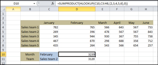
Lookup and summarize a row using the Sumproduct function
In the example (figure 11) 6 months for a specific sales team needs to be summarized. Again as the example above the Sumproduct function can summarize the array. In C11 the name of the sales team is entered. The Excel VLOOKUP is nested inside the Sumproduct function. Col_index_num is many columns (column 2 to 7). Again the curly brackets {2,3,4,5,6,7} is used to tell Excel that it is not only one columns but a number of columns (an array).

Summary – VLOOKUP function
We have covered some detailed aspects of VLOOKUPs and how useful they can be when working with lists and databases. Other instances where you might use VLOOKUPS and HLOOKUPS
- Search Engine Marketing – matching keyword terms, PPC rates, etc
- Sales commission rates – looking up sales for specific rep and applying commission
- Product price/description – looking up a product code to return the price and description
- Stock market data – looking up stock tickers and displaying trading information, stock price, movement


